absolute function

Use of the Absolute function

Introduction

The Delphi "system" unit contains a function called abs( x ) where x may be real or integer.
This function returns the absolute value of x, so

Note, that the abs( ) function combines actually two different functions:

This article focusses on some surprising cases where use of the abs function is time saving and convienient.

1. Distances

While moving the mouse over the screen, (x,y) coordinates are generated.
Say, successive mouseclicks save these coordinates in (x1,y1) and (x2,y2).
We want variables dx and dy to hold the horizontal and vertical distances between points 1 and 2.
This code takes does the job

Note, that there is no difference between the results of abs(x1 - x2) and abs(x2 - x1).

To avoid negative distances, if statements could be used, but this approach is slower.
Modern processors execute instructions in pipelines that read codes ahead.
If statements disrupt this proces, the pipeline has to be rebuild when instruction flow alters.

2. Lower boundery

Say we use a variable x in our program and x is not allowed to be negative.
This means, that a negative value of x must be rounded to zero.
An if statement may do the job, but an abs( ) function can do the job faster.

The understand how this works we first have a look at the graph of the function y=abs(x).

In the above graph the scale is 0.2.
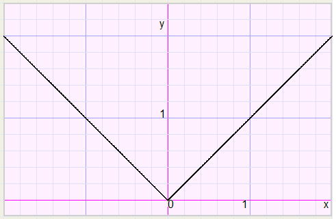
In position (0,0) the graph has a sharp bend.
This is a unique property of the abs function.
Other functions like polynomials, sin, cos, tan, log have smooth graphs, no bends.

All following results are obtained from the above graph.
The bend may not be positioned at (0,0).
Therefore we first introduce a few trics to manipulate graphs in general:
shifting, scaling, reflection.

If in a general function y = f(x) , the x is replaced by (x-1) then
the graph will shift 1 scale to the right.
This is obvious: say point P(p,q) is on the graph y = f(x) , which means that q = f(p).
However if x is replaced by x-1 then not p = x, but p = x -1 is the case so: x = p + 1.
p is changed to p + 1, indicating a shift of 1 scale to the right.
In a similar way we conclude that replacing y by (y-1) shifts the graph 1 scale up in vertical direction.
Replacing x by (x-1) shifts the graph 1 scale left, replacing y by (y-1) shifts the graph 1 scale down.

If in the function y = f(x) , x is replaced by x/2 then the graph will expand by a factor 2 in horizontal direction,
so, relative to the y- axis. (the y axis has the equation x = 0)
similar, if y is replaced by y/2 the graph expands by a factor 2 in the y- direction.

Finally, if we replace x by (-x), the graph is reflected in the y-axis.
Replacing y by (-y) reflects the graph in the x-axis.

With the above knowlegde in mind we may position the bend (0,0) of function y = abs(x).
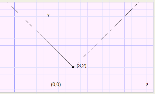
In the graph below

The bend is repositioned at (3,2)

To establish a lower boundary of zero we combine two functions:
y = abs(x) and y = x.
We plot function y = abs(x) + x

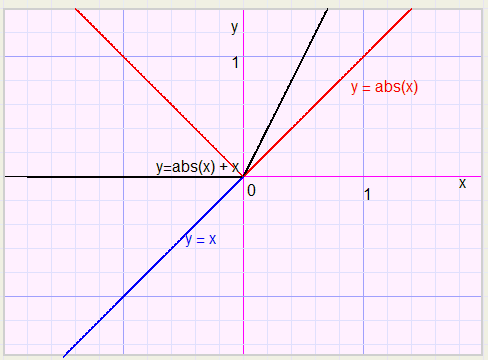
If x < 0 the function sets the lower boundary to zero but if x > 0 the function is too steep (y = 2x, must be y = x).
This is cured by replacing y by 2y, which let the function shrink by a factor 2 in vertical direction.
So the result is

Say, we want a lower boundary of 10, not zero. What to do?
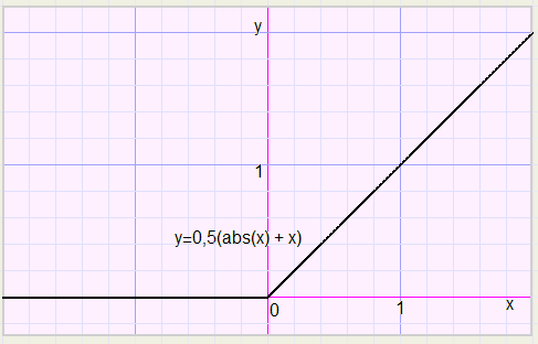
Point (0,0) must be shifted to (10,10).
Therefore we replace x by (x-10) and y by (y-10), so

3.Upper boundary

For an upper boundary we reflect the graph in the y-axis, by replacing x by (-x):

This function yields 0 for x > 0 and abs(x) for x < 0, not quite what we wanted.
Reflection again, now in the x-axis ( y replaced by -y)

Now for x > 0 the upper boundary is zero and for x < 0 we have y = x.
The bending point may be shifted to any position as illustrated before.
The factor 0.5 adjusts the slope.

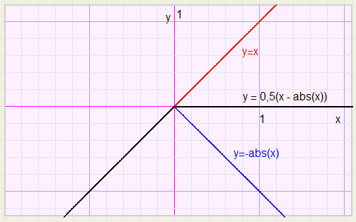
for x = 0 we have reached the upper boundary of 0.
Say we want an upper boundary of 100.
Point (0,0) has to be shifted to (100,100) which is achieved by replacing x by (x-100) and y by (y-100)

4.Upper and Lower boundaries

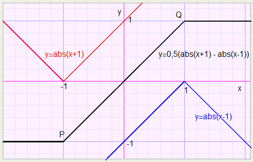
We plot function y = 0,5(abs(x+1) - abs(x-1))
Note: the scale is 0.2

Below x = -1 the function has a lower boundary of -1 and after x = 1 there is an upper boundary of 1.

Note, that abs(lower boundary) = abs(upper boundary) = 1

How to establish other boundaries?
Let's start with function y = 0,5(abs(x+v) - abs(x-v))
For x < -v we may write:

y = 0,5(-(x+v) - (v-x)) = -v ................lower boundary For x > v we may write

y = 0,5((x+v) - (x - v)) = v..................upper boundary And for x > -v & x < v we get

y = 0,5((x+v) - (v-x)) = x ....................no boundary Say we want a lower boundary of a and an upper boundary of b.
The distance between these boundaries is b - a.
So v = (b-a)/2 for temporary boundaries v and -v.
However, the upper boundary is b, not (b-a)/2 so a shift is needed of (end - start), b - v

A function can be build with any lower- and upper boundary.
And without the use of if statements. Pipelines of the processor keep streaming without interruption.
My grapher program Graphics-Explorer may be used to show this results.
Download the program from http://www.davdata.nl/math/grxpl.html
Type y = 0,5(abs(x-a) - abs(x-b) + a + b) and click "plot".
Select (right top) "replace" (not add) and "autoplot".
Left- or rightclick on the a and b fields to change these constants.
Graphics imediately show the new boundaries.

Below I summarize the results (y is the clipped value of x):
Variable x is given

lower boundary a	function	y = 0,5(abs(x - a) + x + a)
upper boundary b	function	y = 0,5(x - abs(x - b) + b)
both boundaries a and b	function	y = 0,5(abs(x - a) - abs(x - b) + a + b)

Quite surprising, isn't it?