

 |
Exponential Curve Fitting |  |
 |
Introduction
This article describes the exponential curve fitting method implemented in Graphics-Explorer.Graphics-Explorer is a function- and equation grapher program, that allows for experimenting
with functions and equations.
By simple mouseclicks points may be added to the screen.
Then the the best fitting poynomial- or exponential function may be calculated.
Calculation of the several type of exponential functions takes place in unit "expfuncUnit".
However, some other units are used, such as the
-
- scaleUnit: supplies scaledY, the distance between two vertically adjacent pixels in the coordinate system.
- least-square unit, which holds procedures
-
- BuildExp12(var PP : puntarray)
- BuildExp3(var PP : puntarray)
Note: punt is Dutch for point. Punten is Dutch for points.
type TPunt = record
              x : double;
	        y : double;
	      end;
var punten : array[1..40] of TPunt;
The complete source code of the ExpFuncUnit you can find [ here ].The following types of exponential functions are supported:
-
1... y = abx + c
2... y = aebx + c
3... y = eax2+bx+c
4... y = abx
5... y = aebx
Note: e is the base of the natural logarithm, e = 2.718.......
A simple general form of an exponential function is..........y = a.gx
For x = 0, y = a, the "start" value.
g is called the growth factor.
Exponential functions are the result of constant relative growth.
Each time x increases by 1, y is multiplied by g.
Note: absolute growth is the result of addition, relative growth is the result of multiplication.
The following graph shows........ y = 10.(0.8)x in red and ........y = (1.1)x in blue.
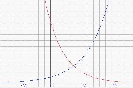
a point x is ....f '(x) ....or...y' , the tangent at (x,y).
The relative speed of growth is f '(x) / f(x) .....or.......y' / y
Exponential functions are usually written in the form.......y = a.ebx, where e = 2.71.....,
the base of the natural logarithm.
Reason is that the function y = ex is it's own derivative, the function y = ex has a constant
relative growth speed of 1.
So, a constant relative growth speed of 1 results in a growth factor of e.
Comparing
-
1....y = a.bx
2....y = a.ebx
The relative speed of growth in 2....is y' / y = b.ebx / ebx = b
Knowing the growth factor g, we may calculate the relative speed of growth being ln(g), since eln(g) = g.
So far this little introduction.
The curve fitting operation will be explained next by discussing a type5 and a type2 curve fitting operation.
Type5: y = aebx
The curve fitting is started by calling procedure expFunc(n : byte), where n = 5.Epower is set true, to differentiate between type4 and type5 functions.
Then procedure exp45 is called.
Exp45 tests for sufficient points, the minimum is 2.
Then procedure getPoints is called to
-
- read all (x,y) points from the "points" unit into array EPoints
- sort Epoints with ascending x values.
Hereafter array Epoints is presented to the least-square unit, which returns the values a and b
in EPoints[1].y and Epoints[2].y.
The buildexp12 procedure is inside the least-square unit and this procedure makes the best fitting
polynomial degree 1 out of the presented points.
Let's look at an example:
Say we have painted points (0,10) and (10,1) on the screen, so
...........Epoints[1].x = 0;... Epoints[1].y = 10
...........Epoints[2].x = 10;..Epoints[2].y = 1.
After the ln ( ) is taken:
...........Epoints[1].x = 0;... Epoints[1].y = 2.302585093
...........Epoints[2].x = 10;..Epoints[2].y = 0.
Procedure buildexp12 makes Epoints[1].y = 2.302585093 = a.... and in Epoints[2].y = -0,230259 = b.
a is replaced by ea = 10.
After that Exp45 builds the formula string with a and b....... y = 10.0 * e^(-0.230259x).
Theory behind:
Having 2 points (x1, y1) and (x2, y2) we may write the system of equations
| | | y1 = a e b x1 y2 = a x b x2 |
| |
| | | ln y1 = ln (a e b x1) ln y2 = ln (a x b x2) |
| |
| | | y1 = a + b x1 y2 = a + b x2 |
| |
In case of more points, the best fitting line is calculated.
a is replaced by ea to cancel the previous ln(a) operation.
Type2: y = aebx + c
This form is more complicated than the previous one, because we cannot take the ln(..) to obtain linear equations.What to do?
Once we know c, the function may be rewritten as ..........y - c = aebx
Then, replacing y - c by y temporarily, we have a type2 function, which was solved before.
How to know c?
It would be nice to have an approximation of c to start with and use a numeric (non analytical) approach to get a more
accurate value of c.
My curve fitter proceeds as follows:
-
differentiation:
y = aebx + c
y'= abebx.........which eliminates c
-
y'1 = abebx1
y'2 = abebx2
...................
(y'2 ) / ( y'1) = eb(x2- x1)
ln((y'2 ) / ( y'1)) = b(x2- x1)
b = ln((y'2) / ( y'1)) / x2- x1)
How to implement this method in practice?
Out of points (x1,y1) and (x2,y2) we make
-
dy = y2 - y1
dx = x2 - x1
y'= dy/dx
because in most cases y' will be more accurate at this point. See figure below.
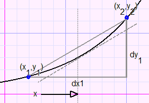
Just as in the case of a type5 function, procedure expFunc(n : byte) is called, now with n = 2.
Epower is set true and makeExpfunction is called.
getPoints extracts the points from the "points" unit and sorts them.
makeExpfunction calls TwoPointsExp if only two points are supplied and calls
morePointsExp if more than 2 points are supplied.
Let's assume 3 or more points are present.
Now the work begins by calling procedure makeXYarrays.
procedure makeXYarrays;
var i : byte;
begin
 for i := 1 to maxpunt-1 do
  begin
   dx[i] := Epoints[i+1].x - epoints[i].x;
   dy[i] := epoints[i+1].y - epoints[i].y;
   dxy[i].x := (epoints[i].x + epoints[i+1].x)/2;
   dxy[i].y := dy[i]/dx[i];
  end;
end;
array dx[ ] holds the difference of the x values of successive points.
array dy[ ] holds the difference of the y values of successive points.
array dxy[ ].y holds the derivative , see figure before.
.........dxy[ ].x holds the x between successive x values.
Note: n points result in n-1 entries in the above arrays
Now, using the method explained above, b is calculated for each pair of sucessive points, so for each entry in dxy[ ].
The b values are added in variable sum, then an average of b is calculated.
Knowing b, we go for an approximation of a.
-
y1 = aebx1 + c
y2 = aebx2 + c.........subtracting.....
y2 - y1 = a(ebx2 - ebx1).............
a = (y2 - y1) / (ebx2 - ebx1)
Knowing a and b, we go for an approximation of c.
-
c = y1 - aebx1
Our temporary goal is reached: an approximation of c.
The a and be values may be forgotten from this point as they are recalculated after the next step:
fine tuning of c.
There is no analytical approach, we have to use a numeric method: successive approximation.
After explaining the algoritm, I shall present an example using real numbers.
There we go.
Instead of y, we use (y - c).
-
(y - c) = aebx
So, if c is accurate, we find this same factor if we compare (y2 - c) and (y1 - c), (y3 - c) and (y2 - c)......etcetera,
because exponential functions are the result of constant growth factors which is constant relative growth.
For a certain value of c, we calculate
-
- the growthfactor comparing two successive points
- the average growth factor
- the (absolute) deviation of the growth factors from the average
function Deviation(cc : double; var af : boolean) : double;
cc is the value of c being tested.
af is the abort flag: true if y = cc intersects (y - cc) = aebx.
-
(y1 - cc) = aebx1
(y2 - cc) = aebx2
so...............
(y2 - cc) /( y1 - cc) = eb(x2- x1)
ln((y2 - cc) /( y1 - cc)) = b(x2- x1)
so...............
b = (ln((y2 - cc) /( y1 - cc))) / (x2- x1)
The growthfactor eb is stored in array growthfactor[ i ]
AVG = eAVG / (xn-1 - x1) is the average growth factor.
Finally, function deviation(..,..) calculates the sum of the absolute differences of each growth factor
and the average value.
Back to procedure morepointsExp. Variable deltaC is the value we increment c with.
If a > 0 , the asymptote will be at the bottom of the coordinate system.
If a < 0 , the asymptote will be at the top of the coordinate system.
(see figure below)
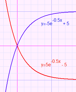
If a > 0 ....deltaC := - scaledY, if a< 0 then deltaC := scaledY.
Incrementing c with deltaC places c further away from the function.
This increment is repeated until procedure deviation(..,..) reports no abort.
Then, deltaC is changed to -deltaC, which makes c move toward the function.
Please look at the flowchart below for the fine tuning of c.
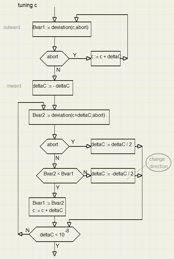
If c is too far away from the curve, moving further away yields a smaller deviation, which would make c run away.
In case of a sharp bend in the curve, the margins for c get smaller.
Hereafter (y - c) is replaced by y which yields a type 5 function and we proceed accordingly.
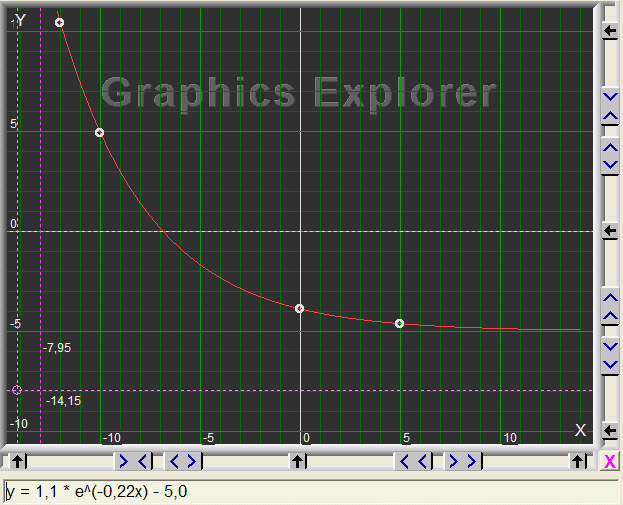
Type5 Example
To test the algorithm, let's take in mind y = 1.1e-0.22x -5.So, a = 1.1, b = -0.22 and c = -5, what we don't tell the computer.
We select 4 arbitrary points (at x values of -12, -10, 0 and 5) on this curve and feed them in the program.
Epoints[ i ].x ; Epoints[ i ].y become:
| i = | Epoints[ i ].x | Epoints[ i ].y |
| 1 | -12 | 10.41452397 |
| 2 | -10 | 4.927514849 |
| 3 | 0 | -3.9 |
| 4 | 5 | -4.633841808 |
the dx, dy, dxy arrays become:
| i = | dx[ i ] | dy[ i ] | dxy[ i ].x | dxy[ i ].y |
| 1 | 2 | -5.487 | -11 | -2.7435 |
| 2 | 10 | -8.875 | -5 | -0.88275 |
| 3 | 5 | -0.7338418 | 2.5 | -0.1467683616 |
Approximations of a, b, c
A first approximation of b results in b = -0.2141An approximation of a = 1.16625
And an initial value of c = -4.977
deltaC is set to -0.05 (scaledY), no intersection, so next: deltaC = 0.05.
Fine tuning c
After fine tuning, c becomes : -5.00000044Linearize Equations
(y-c) is changed to y and the ln(..) is taken to make a, b coefficients of linear functions.Call the least-square procedure
to build the best polynomial, degree 1.Values returned in Epoints[1].y and Epoints[2].y are
..... a = 1.1000004
......b = -0.2199998
These results are rounded by Graphics-Explorer, see below:
 This concludes the description.
