basics of funtion plotting

The basics of Function Plotting

download exerciser program

download Delphi-7 project

see source code listing

This article presents the basics of math function plotting and a Delphi implementation.

The functions are known at design time so we do not need to translate
formulas into basic arithmetic operations taking parenthesis into account.
For formula translation please see fxlate1.

This article focusses on zooming and scrolling.
Also a method is explained to avoid the plotting of asymptotes.

The Coordinate System

The purpose of a (2D) coordinate system is to define the position of points.
For this purpose we use two right-angle lines called the X- and the Y-axis.
The X-axis is generally drawn horizontally, the Y-axis vertically.
Given a point P in the coordinate system, the distance to the Y-axis (horizontally) is called
the X coordinate and the vertical distance to the X-axis is called teh Y coordinate.

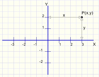
P(3,2) means that point P has distance 3 to the Y-axis and distance 2 to then X-axis.
The intersection of the X and Y axis has coordinates (0,0).

In general, not knowing a specific context, we call the independent variable X and the function value Y.

In this project we use a paintbox to show the coordinate system.
All drawing is done directly in this paintbox.

Below is a reduced image of the paintbox.

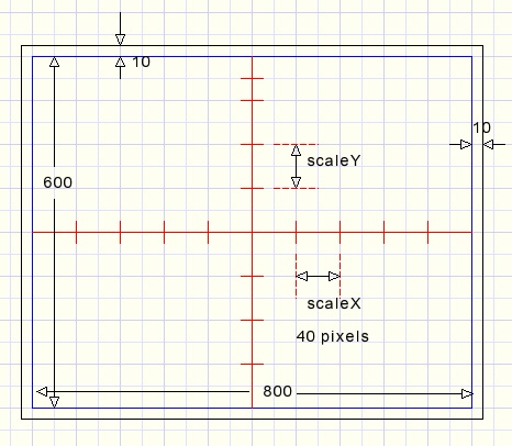
The width is 800 pixels and 10 pixels spacing at the left and right side.
The height is 640 pixels plus 10 pixels at the top and at the bottom.
The raster lines are spaced 40 pixels apart.
X and Y axis are painted in red.

An important pixel is (410,330) which is the center of the paintbox.
Zooming and scrolling is relative to this point.

The following constants and variables define the coordinate system

const maxscalecode = 9;
      minscalecode = 0;
      maxCenter     = 1000;
      minCenter     = -1000;
      scalesBase : array[0..2] of single = (1, 2, 5);
      scalesExp  : array[0..3] of single = (0.01, 0.1, 1, 10);

var centerX : single = 0;
    centerY : single = 0;
    scaleX  : single = 1;
    scaleY  : single = 1;
    scaleCodeX : byte = 6;
    scaleCodeY : byte = 6;
    timercode : byte = 0;
    formulaNr : byte = 1;

scaleX,scaleY is the distance between two horizontal or vertical raster lines,
so the length of 40 pixels.
The default scale is 1. Left- or right mouseclicks in a statictext component alters the scales.
Scalecodes are convenient because they may be incremented or decremented.

The scalecode defines the scale:

scalecode		scale
0		0.01
1		0.02
2		0.05
3		0.1
4		0.2
5		0.5
6		1
7		2
8		5
9		10

centerX, centerY are the coordinates of the paintbox center pixel.
The center values are adjustable as well by mouseclick on the appropriate static text components.
CenterX, centerY are adjusted to be a multiple of the X,Y scales.

Next procedure converts the scalecode to the proper scale value

procedure scalecode2scales;
// scaleCode = scaleBaseIndex + 3*scalesExpIndex
var i,j: byte;
begin
 i := scalecodeX mod 3;
 j := scalecodeX div 3;
 scaleX := scalesBase[i] * scalesExp[j];
 centerX := round(centerX/scaleX) * scaleX;  //make center multiple of scale
 i := scaleCodeY mod 3;
 j := scaleCodeY div 3;
 scaleY := scalesBase[i] * scalesExp[j];
 centerY := round(centerY/scaleY) * scaleY;  //make center multiple of scale
end;

Changing the scales is called zooming, changing the center values is scrolling.

The general way of function plotting

If y = f(x) for every value of x we may calculate y.
This results in a set of (x,y) points and when placed in a coordinate system they show
the relationship between x and y: we see a picture of the function.

Say we calculate f(x) for x values 0, 0.5, 1, 1.5....
First we position the (canvas) pen on point(0,f(0)) then we draw a straight line to (0.5 , f(0.5))
next we draw the line to (1,f(1)) etcetera.

However we deal with pixels, not coordinates.
A translation has to be made between coordinates and pixels taking the scale and center values into account.

Starting with X pixel 10, we calculate the coordinate X value.
This X value is passed to a procedure which calculates the function value.
The function value is passed to a function which converts this coordinate Y value to a pixel position.
Then the procedure repeats for horizontal pixel 11.....etc.
Straight lines are drawn from one pixel to the next.

This function converts a horizontal pixel value to the coordinate value

function pix2X(px : smallInt) : single;
//pixel value px to x value
begin
 result := centerX+0.025*(px-410)*scaleX;
end;

Following function converts a Y coordinate to it's pixel Y position

function getPixelValue(y : single) : smallInt;
var pixY : single;
begin
 PixY := 330 - 40*(y-centerY)/scaleY;
 if PixY < 0 then pixY := -1;       //avoid integer overflowing
 if PixY >= 660 then PixY := 660;
 result := round(PixY);
end;

Notice that at first a floating point value (pixY) is used for the pixel position.
This avoids overflowing of the integer result.
So far, many functions may be plotted but not all.

Floating Point exceptions

Some floating point operations result in errors.
Division by zero and the attempt to take the square root out of a negative number
are the main causes of floating point exceptions.
What to do if this happens during function plotting?
The answer is simple: nothing.
We may only draw lines when we obtain valid floating point values.
Therefore the calculation of the function value also returns a (v) flag
indicating the validity of the result.

At a valid value we may position the pen, at a following valid value we may draw a line.
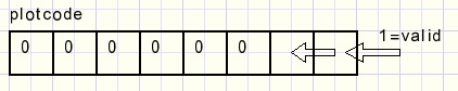
To control this proces there is a variable plotcode

This function calculates the value of the selected formula

function getValue(x : single; var v : boolean) : single;
//calculate function value
var sqx : single;
begin
 result := 0;
 try
  case formulaNr of
   1 : result := 0.1*x*x-6;
   2 : result := sqrt(64-sqr(x));
   3 : begin
        sqx := x*x;
        result := sqx*(-0.01*sqx +0.5);
       end;
   4 : result := 1/(x-2.001);
   5 : result := 5/((x-4.001)*(x+3.999));
  end;//case
  v := true;
 except
  v := false;
 end;
end;

This code does the drawing:

var px,py : smallInt;
    x,y : single;
    plotcode: byte;
    valid : boolean;		
begin	
with form1.plotbox.canvas do
............
 for px := 10 to 809 do
  begin
   X := pix2X(px);
   Y := getValue(x,valid);
   if valid then py := getPixelvalue(y);
   plotcode := (plotcode shl 1) and $3;
   if valid then plotcode := plotcode or $1;
   with form1.plotbox.Canvas do
    case plotcode of
     1 : MoveTo(px,py);
     3 : lineto(px,py);
   end;//case
  end; //for px

Asymptotes

There is one other pitfall.
Imagine the function y = 1/x
For x = -0.001 y = -1000.
For x = 0.001 y = 1000.
The line x = 0 is called an asymptote.
We do not want the drawing of asymptotes as they do not represent valid function values.
When asymptotes coincide with the coordinate system raster, the valid flag will drop because
we generate infinite floating point values.
The asymptote will not be drawn in this case.
The function y = 1/(x-0.01) however has asymptote x = 0.01 and
for a horizontal scale of 1 (0.025 per pixel), this happens:

Without extra checks and precautions, the line from (0, -100) to (0.025, 66.67) is drawn erroneously.

What to do?
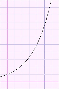
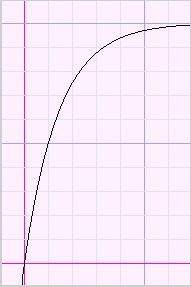
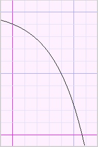
Please look at the function plots below:


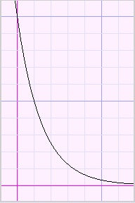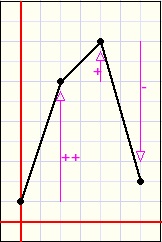
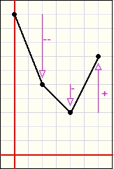
inc. ascent	dec. ascent	inc. descent	dec. descent

We notice functions which ascent increasingly, ascent decreasingly,
descent increasingly or descent decreasingly.

This behaviour is described by the derivatives of the function.
Between two sucessive pixels (x1,y1) and (x2,y2) the derivative is (y2-y1)/(x2-x1).

Now consider three successive pixels with values (x1,y1) (x2,y2) and (x3,y3).
Because the horizontal pixel distance is the same,
for comparison of the derivatives we may assume (x3-x2) = (x2-x1) = 1.
Then the derivatives are (y2-y1) and (y3-y2).
So the derivative is positive for an ascending function and negative for a descending function.

The so called second derivative is the difference between derivatives : (y3-y2) - (y2-y1).
For an increasingly ascending function, the first and second derivatives are both positive.
For a decreasing descending function the first derivative is negative but the second is positive.

Now comes the tric.
If we calculate the y values for three adjacent points and the two derivatives have the same sign
(both positive or negative) we may draw the two lines between these points.
If the derivatives between points have unequal signs however, we observe the second derivative
calculated for the three previous points.
If this first and second derivatives have unequal signs, the function value is set invalid.


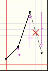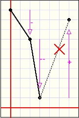no plot	OK	no plot	OK

Below is the complete plotting method:

procedure TForm1.plotbtnClick(Sender: TObject);
var x,y,prevY,dY,prevdY,ddY : single;
    valid,OK : boolean;
    plotcode : byte;
    px,py : smallInt;
begin
 plotcode := 0;
 py := 0;
 prevY := 0; prevdY := 0; ddY := 0;
 with form1.plotbox.Canvas do
  begin
   pen.Color := $000000;
   pen.Width := 1;
  end;
 for px := 10 to 809 do
  begin
   X := pix2X(px);
   Y := getValue(x,valid);
   if valid then py := getPixelvalue(y);
   dy := Y-prevY;
   if dY*prevdY >= 0 then OK := true        //asymptote suppression
    else OK := dy*ddy >= 0;
//   OK := true;                            //OK=true allows drawing asymptotes
   valid := valid and OK;
   plotcode := (plotcode shl 1) and $3;
   if valid then plotcode := plotcode or $1;
   with form1.plotbox.Canvas do
    case plotcode of
     1 : MoveTo(px,py);
     3 : lineto(px,py);
   end;//case
   ddY := dY - prevdY;
   prevdY := dY;
   prevY := Y;
  end; //for px
end;

Y		function value of last point.
prevY		function value of previous point.
dY		derivative Y-prevY.
prevdY		previous derivative obtained by second and third last points.
ddY		second derivative dY-prevdY.

This concludes the description.