Equation grapher description

Equation Grapher description

Introduction

In a previous article

I discussed how functions or equations are dissected
into basic arithmetic operations allowing the value to be calculated.
The result was the Director Table, which is a list of basic arithmetic operations sorted from high to low priority.

To plot the functions I included unit eqdrawer and it's code is described below.
Note:

So, a function is a special form of an equation.
functions are used widely because, yielding only one result, they may be used in formula's.
An example is y = 3sin(x).

In the fxlate project, 4 type of functions or equations are supported.
The options to draw the graph are intentionally kept very simple because the only purpose
here is to illustrate the proper translation.

The coordinate system is in paintbox1 on form 1, the size is 640 * 480 pixels.
The origin of the coordinate system is at pixel position (320,240).
The domain of x is -8 ... + 8, the domain of y is -6...+6.
The scale is fixed to 40 pixels per cm.

In general, equation plotting is calculating consequetive (x,y) number pairs and connecting them by straight lines.
Keep in mind, that certain values of x, y result in arithmetic errors if we try to calulate the square root or logarithm
of a negative number or if we divide by zero.
The calculate(var OK : boolean) procedure will set OK to false in this case and the plotting software must act accordingly.

Supporting functions

Below I discuss the drawing procedure per function type.
Refer to the eqdrawer source code for more details.

Type1 functions {y = ......x........}

Variable i is incremented from 0 to 639.
i is converted to a x value by calling pix2x(i).
Then setX(x) sets x and calculate(valid) is called to calculate y.
y := getY yields the calculated value of y.
Counter vcount represents the number of valid points received. It counts 0,1,2,2,2...
At value 1, a moveto(i, y2pix(y)) takes place, at vcount = 2 a lineto(i, y2pix(y)) takes place.
If valid = false, vcount is reset to zero.
Also a check is made for the difference of two consequetive y values: if too large, painting is suppressed.
This avoids painting asymptotes as in y = tan(x).
This asymptote suppression is somewhat primitive, more sofisticated but more complicated procedures are possible.

Type2 functions {x = ......y........}

Basically the plotting is the same as for type1, but x and y are traded.

Type3 functions {y = ..v...; x = ....v...}

Here, i runs from 0 to 400 and v := 0.025*i.
This choice is based on the interval 0..2*pi for trigonometric functions, allowing the paint of Lissajous figures.
After calling the calculate(var OK : boolean) procedure, getX and getY are the calculated x and y values.
vcount takes care of the lineto(..,..) and moveto(..,..) methods.

Type4 functions {...y...x... = ...x...y...}

This procedure is a little more complicated than the ones before.
Remember, that a type4 equation is of the form ....x....y.... = ...x.....y...
and may become rather complicated.
Try for instance (x^2 + y^2)(y^2+x(x+5)) = 20*x*y^2....which yields a trifolium.

In the translate process, this equation is changed into v = (x^2 + y^2)(y^2+x(x+5)) - 20*x*y^2
where - is given a priority of 2 and = of 1.
Therefore, after settting x and y and calculating, v will be zero if values left and right of the original
equation are the same.
Plotting proceeds as follows:
Calculate v for every pixel in the coordinate system.
If v = 0 , plot the pixel.
If v changes sign between two horizontal or vertical pixels, plot the pixel with the smallest absolute value.
Note, that in floating point calculations answers may be 0.0000003 or so instead of 0 due to rounding.
Also, pixel positions not necessarily are nice integer values.

Also note, that this method of plotting may produce the graph of very complicated equations,
but the speed of drawing is much slower than of the type1,2,3 functions.

Variable i steps horizontally from 0 to 639, j steps vertically from 0 to 479.
Say, we have just processed line j.
v is an array[0..639] of double, that holds all calculated values of v for an entire row j of pixels.
code is an array[0..640] of byte holding information about v[..]:

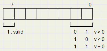
For new line j+1 v is calculated for a value of i. The value is stored in variable nextV.
The code is stored in nextcode.
Then a logical and function: nextcode and code[i] takes place.
If the result = $80, then both pixels v[ i ] (at row j) and nextV at column i of row j+1
are valid and show a change in sign.
The pixel with the smallest absolute value is then plotted.
After this, v[ i ] := nextV and also code[ i ] := nextcode.
If the complete row is done, v[ ..] holds the values for row j+1 and this line is now examined
for codes of $83 (zero results) or sign changes.

At the start of the pixel scanning process, code[0..640] is set to zero.
Thus, while reading row 0, no sign change can be detected between vertically adjacent pixels.
By extending the code array to 640 instead of 639, the highest column, the check for sign changes
in a row is made easier because the comparison is made between [ i ] and [ i+1 ] where i runs from 0..639.

This concludes the description of graphs painting.